How I used Dijkstra’s Algorithm To Find An Optimal Route To Work.

In this article, I would like to share my experience and experimentation of using Dijkstra’s “Shortest Path” algorithm to figure out an optimal route to travel everyday to a new job on the other side of the city.

I did a few modifications in the edge cost calculation to include factors beyond just distance, so it is not really the shortest path that I wanted, but more of a comfortable path that was optimized for me.

The Context:

Recently, I changed my job and the most imminent problem I had to face was travel. I am used to staying near my workplace and have worked for a couple of companies within walk-able distance from my place of residence, for over 3 years.

Before you start to judge me and call me lazy, staying close to one’s workplace is a logical thing to do in the city I live in, which is Bangalore, notorious for its traffic and road congestion.

I really didn’t want to waste a lot of time, travelling every day.

But I guess I was lucky because this problem actually turned out to be an opportunity in disguise to improve and hone my problem-solving skills. An opportunity to come up with and apply some algorithm for a real-life situation. That sounds exciting, isn’t it?

Here is a link to a quick refresher on the actual Dijkstra’s algorithm.

The Modification:

The actual algorithm considers the edge costs between nodes as the distance between the nodes being considered.

In my case, the distance was not the only concern. There were other factors in addition to it such as:

The traffic density on a specific route.
The comfort level of the means of commute.
The actual commute duration itself.

So, based on these, it made more sense to weigh the edges using a normalized value that considers the above factors as well in addition to the distance.

Like I mentioned at the beginning of the article, I was trying to figure out an optimal path that I would be comfortable with and not the shortest path.

This subjective nature of the problem is what makes it more interesting in my opinion. Because real-life human-centred issues cannot be solved with pure logic alone but require a lot more, such as intuition and empathy.

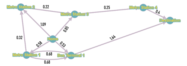
The Graph:

Since my preference is to use public transportation facilities, the graph nodes were constructed based on the routes that were actually serviced by one or more of the public transportation modes.

The Weight Ratio:

As discussed above, based on my subjective preferences, I came up with the following rating that would yield an optimal route that I will be comfortable with.

The edge weights will be a normalized number based on the following distribution:

Distance: 40%

Traffic Density: 50%

Travel Comfort: 2%

commute Duration: 8%

The final factor of commute duration might be a bit confusing because one might think that it would be directly proportional to the distance. so why one should bother considering it?

This is true for most cases. But in my case, since I prefer the public transportation options, the factor will not always be proportional to distance.

The speed of commute of each mode offered by public transport corporations vary. For example, a train will have a lesser commute duration than a bus on the same route for the same distance.

If a shorter route doesn’t have a train option but another longer one has it, there is a possibility that taking the train on the longer route might get me quickly to the destination because of the drastic reduction in traffic density and increase in commute speed. Also, it might be having a higher level of comfort than a crowded bus. Hence decided to consider it as a factor.

A simple Formula:

So, the edge cost calculation would be like:

The distance is the physical distance by road or rail track between two nodes in kilometres.

The traffic density is measured on a scale of 0 to 10 where 0 means no congestion and 10 being fully congested for more than 30 minutes.

The comfort level is a very subjective measure on a scale of 1 to 10. This metric depends on how crowded the mode of transport is, whether one could travel seated and the availability of air-conditioned carriers on the route.

commute duration is the average of the actual time it takes in minutes to travel between the nodes.

To reduce the bias in data, all the numbers used for calculation were averages of data recorded during a span of three weeks travel at peak hours of traffic.

Also, while recording the commute duration metric, I included the waiting time incurred for the mode of transport.

Applying Costs To Edges:

After the data collection process on the identified routes, it was time to apply the formula to calculate the edge costs and complete the graph.

By applying these values to the above-mentioned formulae, the cost of each node was determined. Unlike the actual Dijkstra’s algorithm, I decided to have the cost in decimals rather than integers.

Thus the weights were added to edges as follows:

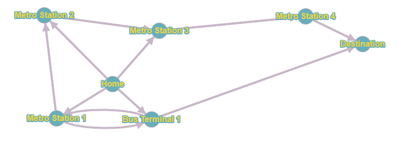
The Algorithm:

Now that we have the entire data organized in a graph with nodes and weighted directed edges, it is simpler to apply Dijkstra’s shortest path algorithm on it.

Conclusion:

It is always a delight to know that we can apply many computer science concepts in real life for human situations to find a solution.

The world is full of possibilities and we could optimize it to our own needs as we would do while developing a performant software system. I guess curiosity is the key.

If you are wondering, I actually found an optimal route that suited me, using the algorithm described above and travelled through it for a week. But staying closer to the workplace was the most efficient solution for me. So I shifted after that week.

Maybe I shall write another article at a later time on how I used the “Optimal Stopping” concept to rent a place pretty quickly near my new workplace.

Thanks for reading my thoughts,

cheers :)